If somebody asked the author of this website if they were allowed one computer with only two applications installed, and no more, then which two they would be? The answer would be simple: A web browser and a copy of Microsoft Excel. Whilst familiar with all of the other Microsoft Office applications, a reasonable knowledge (from previous work) of Adobe programs, such as InDesign, Photoshop and Fireworks, and countless other applications, nothing surely beats Excel for versatility.

Above: Excel launcher icons throughout the years. How far back can you remember? The first versions of Excel came out in 1985 (Mac) and 1987 (Windows).
The purpose of this webpage is not to provide a comprehensive tutorial in Microsoft Excel, rather than to maintain a personal record of some of the tools and tricks the author has found out whilst using Microsoft Excel throughout the years; thus, this webpage is not intended to “reinvent the wheel”. There follows no “how-to” instructions, rather just a selection of task-specific tips which the author found useful along the way.
Creating a Dropdown List
Starting with some basic features, the dropdown list is useful with ensuring data input is consistent with a choice of entries and helps with eliminating typing errors where required input can be pre-defined.
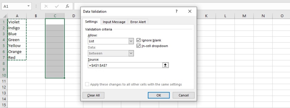
In this example, cells in column C are highlighted, under “Data”, “Data
Validation” is selected, then under “Allow:”, “List” is selected, and
the Source is selected as cells A1 to A7. Then a custom error alert can
be set to stop entry other than one of the listed colours, with a
message alerting the user, if their cell input does not match one of
them.
The data validation tool can also be used to put certain restrictions on
what is entered into specified cell. For example, a date entry within a
specific range or after a specific date, or a numerical value only to a
specified number of decimal places. This can help with the accuracy of
information entered onto a spreadsheet. Validating data input (as well
as number formatting) can also help later with ensuring it is fit for
calculations and/or presenting in a consistent format.
Rounding Numbers
Rounding numbers using the formula =ROUND(number, num_digits) is important if applying IF formulas to compare a value against a specification. For example, if a value is always reported to one decimal place, there is no use in comparing a value of 8.03 with a specification of 8.0; the IF formula will state that 8.03 is greater than 8.0. However, if the 8.03 is rounded to 8.0, it will not be greater than the specification (in any circumstances where rounding up is always necessary, the ROUND function can be replaced by the ROUNDUP function).
VLOOKUP (& Some Other Basic Formulae)
An extremely useful tool in retrieving data from a table is the VLOOKUP formula. Building on the previous example, the image below lists some vehicles in column B and their colour, as selected from a dropdown list, in column C:
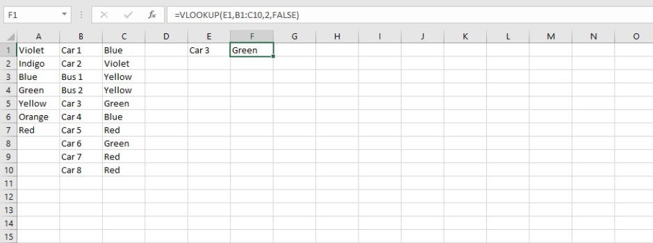
In E1, the name of a vehicle listed in column B is entered. In cell F1, the following formula is entered:
=VLOOKUP(E1,B1:C10,2,FALSE)
Where E1 is the value to look up, B1:C10 is the range to search, and 2 = the column number of the range to return the value from. The parameter of FALSE means that VLOOKUP is looking for an exact match for the value (TRUE would mean that an “approximate” match would be used with respect to returning a data value). And so here, because E1 contains the text “Car 3”, cell F1 has looked in the appropriate cells and returned its corresponding colour, Green.
Note 1: If, for example, Car Number or Bus Number ha been entered twice in column B, then the VLOOKUP formula would return the first value it finds, as it searches down the list. For this reason, I would set up a table where the vehicle and its number are initially entered, and have a separate list, where duplicate entries are eliminated, next to which the colour would be entered. This can be achieved using the “COUNTIF” function.
Note 2: If there is no entry for colour, then the value zero might be returned. This issue can be eliminated by embedding the VLOOKUP formula into an IF statement, whereby if the VLOOKUP value zero is returned, “Not Determined” is displayed. Also, when using VLOOKUP formulae, sometimes there may be errors returned in the cell, in which case, I “tidy up” the spreadsheet by embedding the VLOOKUP formula into an ISERROR statement in addition, or instead (ISERROR checks if the returning value is an error or not).
Note 3: Once a spreadsheet is created, it is always useful to lock all cells with a password, other than those where data is to be entered, to help protect those all-important formulae!
Examples where I have used a combination of VLOOKUP, IF, COUNTIF and ISERROR formulae, as well as others, such as “NOW”, which returns the current date and time, include creating Laboratory Information Management (LIMS) systems, where data generated is maintained and accessed in a database (Microsoft Excel provides a more versatile means of performing numerical calculations on data than database programs, such as Microsoft Access), maintaining inventories of items which have an expiry date, keeping staff holiday records and ensuring there are no clashes with other members of staff trained in the same procedures who have already booked time off, and maintaining medication stocks of clients/reordering forms within a residential care home setting. These are just a few examples and, of course, the number of possible applications using these formulae is seemingly endless.
Removing Repeat Entries from a Single Column (e.g. Batch or Lot Numbers)
If, for example, information is to be recorded for items with unique reference numbers (e.g. data pertaining to a batch in this example, or lot number), it may be essential that a row of batch information is not repeated in the spreadsheet. Simple formulae may be used to ensure that each batch number is entered only once. For this example, formulae may be altered where applicable, including adjustments if the data is presented in a transposed format. Some of the description below may seem a bit tricky at first, but once the formulae have been entered into a spreadsheet, things should hopefully make a bit more sense if they didn’t first time.
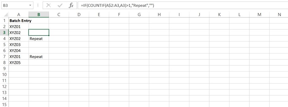
In the example above, batch numbers are recorded in column A, and column B highlights repeated entries by returning the word “Repeat”. Cell B2 is left blank as the first entry under Batch in column A cannot be a repeat. Cell B3 contains the formula =IF(COUNTIF(A$2:A3,A3)>1,"Repeat","") . You will see that there are two formulae being used here. The COUNTIF is looking at the range A2:A3 and counting the number of instances where the entry in cell A3 may be found. The IF statement is then returning a true value (=”Repeat”) if the number of instances of the entry in column A is greater than 1 (i.e. if it is a repeated batch number entered). The purpose of the $ in the formula is to keep the value 2 in the range A$2:A3 fixed when dragging the formula down to extend the table. And so, dragging down the formula in cell B2 will change the range of cells being looked at to A$2:A4, A$2:A5, A$2:A6… and so on. The value being checked to see it is being repeated will always be that in the cell to the left of the cell the formula is entered into.
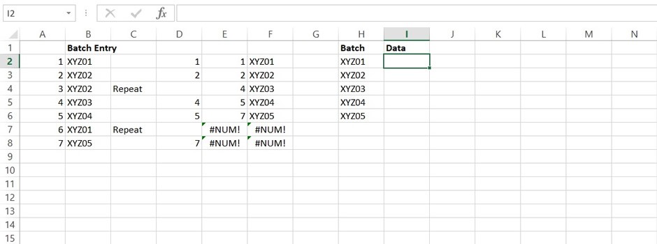
Following on, we may now wish to have a neat list of all the entries without the repeat values and without blank rows (as seen in column H, above). In this example, the left area is set aside just to enter batch numbers in. On the right hand side (Column H,I,J etc.), batch numbers, minus repeats, can be displayed (preferably in locked cells), ready for Batch information to be entered horizontally (as mentioned above, all of this can be transposed if desired so that batched go across and data down. However, it is worth noting that Excel spreadsheets have many more rows than columns).
And so, for sorting, the following technique may be used (there may be
other ways). First, I have inserted another column to the left of the
batch number entry column and entered incremental numbers for each row.
Cell D2 contains the formula =IF(C2="",A2,"") . Here, it will display a
number from column A, only if the Batch entered is not a repeat. The
cell D2 formula can be dragged down.
Cell E2 contains the formula =SMALL(D$2:D8,A2). This will return the
smallest value in column D (A2 equalling 1). The Cell E2 formula can be
dragged down. Cell E3 contains the formula =SMALL(D$2:D9,A3). As A3=2,
it will show the second smallest value in column D. Subsequent rows in
column E will return the third smallest value from column D, then the
fourth smallest and so on.
Cell F2 contains the formula =VLOOKUP(E2,A$2:B8,2,FALSE) . Here, the
value in cell E2 is searched for in the range A2:B8, returning the value
in the second column of the row where it is found. You will see, we now
have a list of the batches entered, without repeated batch numbers and
with no spaces between them. Again, this formula can be dragged down.
Note that the B8 may be extended and amended to B$1000, or however large
the spreadsheet is anticipated to be.
Finally, cell H2 contains the formula =IF(ISERROR(F2)=TRUE,"",F2). This
is also dragged down and in essence returns the same values as those in
column F, minus any error values which may be displayed where there is
no batch number to return. Note: If using a spreadsheet which is
transposed w.r.t. this example, the HLOOKUP formula may be used in place
of VLOOKUP.
Returning the nth (or nth to nth) Value(s) Using the MID Function
The Mid formula is in the form =MID(text, start_num, num_chars)
This can be useful if it is required to extract characters from a cell
entry, where the position of those characters will be fixed. For
example, if we wanted to return A or B from the following data:
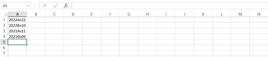
In cell B2, we could type:
=MID(A1,5,1)
This will return “A” in cell B1. The formula can be dragged down the
column for the rest of the entries in the spreadsheet.
By typing =MID(A1,5,2) in cell B1, the values “Av” will be returned.
Playing with Numbers and Letters
Sometimes it may be necessary to tidy up data. For example, if routinely importing .csv files from an external source into a pre-formatted Excel template. Some of the following formulae may be of help:
Removing the nth characters from a cell entry:
=REPLACE(old_text, start_num, num_chars, new_text)
From the previously shown example, by entering the following into cell
B1:
=REPLACE(A1,1,4,"")
The value “Av22” will be returned in cell B1
Note: this formula can be used to replace the characters with something
else, by substituting the “” in the formula with what it is to be
substituted for.
Replacing specific text from a cell entry:
This can be achieved using the formula
=SUBSTITUTE(text_string,old_text,new_text)
So, entering =SUBSTITUTE(A1,"A","X",1) into cell B2 would
return”2022Xv22” (from “2022Av22”)
Note: this formula can be used to remove specific characters, by
substituting the “new_text” in the formula with “”.
SUBSTITUTE replaces one or more instances of a given character or a text string, whilst REPLACE changes characters in a specified position of a text string.
Extracting left (or right) characters:
The LEFT function or the RIGHT function extract a substring from the
left or right side of a text string respectively:
=LEFT(text,[num_chars]) or =RIGHT(text,[num_chars])
So, for example, using the example shown in the previous image, if
=RIGHT(A1,3) were entered into cell B1, the value “v22” would be
returned in cell B1
Reporting to Significant Figures
In some situations, values may be reported to a number of significant figures, as opposed to a number of decimal places. Values may be reported this way as per the following example:
=ROUND(A1,3-(1+INT(LOG10(ABS(A1)))))
Where the value in cell A1 is to be reported to (as an example) 3 significant figures. (3 can be replaced by another value or by a cell reference, if the number of significant figures to report to varies)
Hiding Formulae Where the Returned Value is for Calculation Purposes Only
In a number of instances, in order to simplify things and prevent the creation of very long formulae that can appear confusing to anyone else editing the spreadsheet formulae, a calculation may run over multiple cells using different formulae in each step of an overall calculation. In this situation, it may be desirable to hide intermediate calculation steps from an end user, so as to make the spreadsheet look more user-friendly, tidier, and also more presentable, especially if printing. One common way is to simply hide a column (or row) using the Hide option in Excel. Other than recolouring text to white (or whatever the cell fill selected is), a much more convenient way is to simply set a custom format of the cell(s) containing the formula(e) to be hidden to three semicolons (Format Cells, Number Tab, Category: Custom, Type: ;;;).
Returning the Sheet Name in a Cell
This can be achieved using the following formula (in a workbook that has already been saved somewhere):
=MID(CELL("filename",A1),FIND("]",CELL("filename",A1))+1,255)
Presenting Tables of Read-Only Data on a Webpage
This is another use I have found for Excel. A workbook containing information (only) in tables in Excel is saved as a webpage. The first worksheet is then added to a webpage using an iframe in HTML and the other worksheets can be viewed in the webpage as displayed in a browser, by clicking on the different worksheet tabs, as one would do in Excel itself.
Protecting / Unprotecting all Worksheets
For protecting all worksheets in a workbook, run the following in Visual Basic for Applications (VBA):
Sub
ProtectAllWorksheets()
Dim ws As
Worksheet
Dim Pwd As
String
Pwd =
InputBox("Enter your password to protect all worksheets", "Protect
Worksheets")
For Each ws In
ActiveWorkbook.Worksheets
ws.Protect Password:=Pwd
Next ws
End Sub
For unprotecting multiple worksheets in a workbook, run the following in Visual Basic for Applications (VBA):
Sub
UnProtectAllWorksheets ()
Dim ws As
Worksheet
Dim Pwd As
String
Pwd =
InputBox("Enter the password to unprotect all worksheets", "Unprotect
Worksheets")
On Error Resume
Next
For Each ws In
Worksheets
ws.Unprotect Password:=Pwd
Next ws
If Err <> 0
Then
MsgBox "Incorrect password entered. All worksheets could not " &
_
"be
unprotected.", vbCritical, "Incorect Password"
End If
On Error GoTo 0
End Sub
Using Excel for Drawing
For all of its power in handling numerical data, Excel can be surprisingly useful when it comes to drawing. Not only for flow-charts and the like, but as seen here, it is a useful tool for scaled drawings. The use here, came in the form of creating diagrams of Orreries (models showing the rotation of planets around a star, or moons around a planet) which were constructed out of Meccano. An example is shown here:
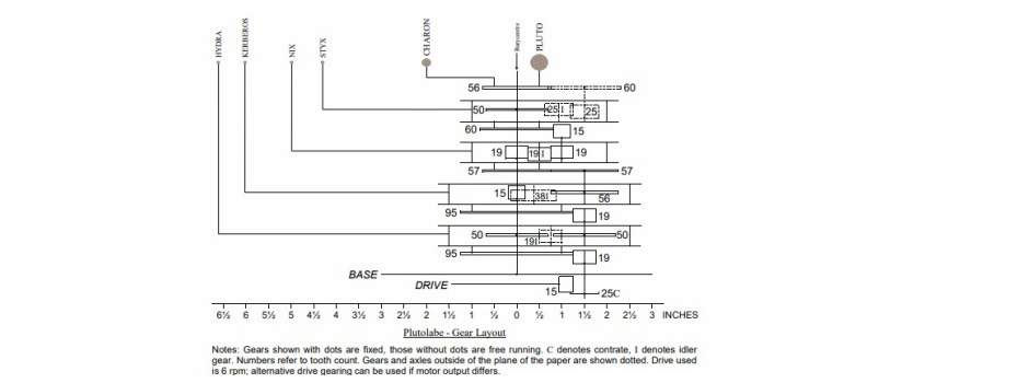
Prior to creating the drawings, which involved using cell borders for the horizontal and vertical lines, for this purpose it was necessary to make the cells on the worksheets square. This can be achieved by selecting “Page Layout” under the “View” tab. Column widths and row heights will now be in ruler units (inches, centimetres or millimetres, depending on how your version of Excel is set up). Then, adjust the row heights and column widths to an identical value as seen fit. By changing the view setting from “Page Layout” back to “Normal”, row heights and column widths will be displayed in points again.
Note: To change the ruler units visible in Page Layout (e.g. from mm to inches or vice versa), then under “File”, select “Options”, then “Advanced” and under the heading “Display”, change the Ruler units using the dropdown menu and click on “OK” to apply.
How to Get Directory/Folder Names and File Names from File Manager/Windows Explorer into Excel
In a situation where there are a large quantity of files and folders stored on a computer and the names of them all need to be recorded, I have written a guide on how to do this (in Windows). Note – for the filenames, see Note 2 on page 4. The guide can be viewed on the link Here.
Back to Top